From Kafka to Amazon S3: Partitioning Outputs
So you’ve got a ton of data that needs to be processed in real-time, huh? Don’t worry, in this tutorial I’ll show you how to stream data from Kafka compatible streaming platform to Amazon S3.
But wait, there’s more! I’ll also cover how to create partitioned outputs, which allows you to organize your data into separate files based on a chosen partitioning key. This is especially useful for scenarios where you want to query or analyze data based on specific attributes, such as timestamps or geographical locations. By partitioning your data, you can easily access and analyze subsets of your data without having to process the entire dataset.

Kafka is a distributed streaming platform that can handle massive amounts of real-time data, while S3 is a cloud-based object storage service that can store and retrieve data at scale. I’ll show you how to combine these two powerful tools to create a data processing pipeline that’s fast, reliable, and scalable. Whether you’re working with financial data, social media feeds, or IoT sensor data, this tutorial will help you get started with streaming data from Kafka to S3.
So grab a cup of coffee (or your favorite energy drink) and let’s dive in.
Problem statement
Organizing data is not exactly the most exciting thing in the world. But if you’re working with a large dataset, you know that keeping everything in one place can quickly become a nightmare. That’s where partitioned outputs come in. By dividing your data into smaller, more manageable chunks based on a chosen partitioning key, you can finally have some control over your data.
Let’s say you’re working with a dataset of customer transactions and you want to partition the data based on the transaction date. You could create a partitioned output structure where each partition corresponds to a specific date, with files containing all the transactions for that date. For example, you could have the following partitioned output structure for the month of March:
s3://my-bucket/transactions/year=2023/month=03/day=01/
s3://my-bucket/transactions/year=2023/month=03/day=02/
s3://my-bucket/transactions/year=2023/month=03/day=03/
…
s3://my-bucket/transactions/year=2023/month=03/day=31/
In this example, each file within a partitioned directory would contain all the transactions for that specific date. You could also add additional levels of partitioning for other attributes, such as the customer ID or the type of transaction. The advantage of this method is that with this structure of files if you need to find a corrupted file for March 2 or delete all user transactions for the entire March it will take a couple of seconds.
Another example, you have a JSON data stream containing customer orders with each order having a unique order ID. You want to partition the data by order ID so that you can easily retrieve orders for specific customers and analyze their purchasing behavior.
To achieve this, you can configure your application to write each order to a unique S3 object based on its order ID. For example, you could use the order ID as the key for the S3 object and store each order as a separate file within that object. So, for an order with ID “12345”, you might store it in an S3 object with the key “orders/12345/order_data.json”.
When you want to retrieve orders for a specific customer, you can simply query the appropriate S3 object based on their customer ID and retrieve all the orders associated with that ID.
By partitioning your data, you can significantly reduce processing times and make data analysis more efficient.
What we’re going to use in this tutorial
So, for this tutorial, we’re gonna use a Kafka-compatible platform called RedPanda. Why? Because it’s like Kafka, but with a fancy name and much faster.
We’ll also want to run this tutorial on our local computers, so we’re going to need Docker, Docker Compose and a bit YAMLs. Since we don’t want you to spend a fortune on AWS S3 storage, we’ll be using the budget-friendly alternative, MinIO. And to tie it all together, we’ll be using Kafka Connect, the middleware that helps us move data between Kafka and other systems. With Kafka Connect, we can seamlessly push data from Kafka topics to external storage systems using pre-built connectors called “sink connectors.”
In fact, Kafka Connect has sink connectors to different cloud platforms like Google Cloud Storage, Microsoft Azure Blob Storage, and more that you can find here, but we’re going to use Amazon S3 for this tutorial because it’s a very popular choice for data storage with its virtually unlimited storage capacity and pay-as-you-go pricing model.
This tutorial is divided into three parts, each covering a different aspect of streaming data with Kafka Connect. In the first part, we will explore how to stream simple JSONs using the DefaultPartitioner, which preserves the default Kafka topic partitions. In the second part, we will dig into more advanced partitioning techniques by using FieldPartitioner and TimeBasedPartitioner to create partitions by selected field or timestamp. Finally, in the third part, we will use Confluent Schema Registry to stream binary data in Protobuf format and convert it to Parquet on the fly. By the end of this tutorial, you will have a good understanding of different partitioning techniques and how to use them in your Kafka streaming applications.
Setting up the environment
So let’s get started, shall we?
This tutorial is designed for MacOS users, so the first step is to install Docker Desktop. After that, we can create YAML configuration files to set up our local environment.

If you’re not familiar with Docker and Docker Compose, I recommend going through the official tutorials: Docker tutorial and Docker Compose getting started article. Additionally, here’s a recommended Docker course for those who need further guidance.
Alright, let’s split our work! We will create a shared Docker Compose YAML file for all three cases and individual YAML files for each case that will contain the required Kafka Connect configurations and any additional services specific to that scenario. This will help us avoid unnecessary duplication and make it easier to manage the entire setup. With this approach, we can easily switch between different scenarios.
This docker-compose file below sets up a streaming data pipeline with RedPanda, RedPanda Console as the management UI, MinIO as the object storage server, and AWS CLI as the tool to interact with the object storage server.
Let’s look at the schema below to understand what we got here with this YAML.

Here, we have a RedPanda instance with a pre-created test topic, a MinIO instance with a pre-created “my_bucket” bucket, access to the pipeline through the RedPanda Console, and a Kafka Connect instance that will consume data from the test topic and upload it to the “my_bucket” bucket. Throughout the tutorial, we will only change the configuration of Kafka Connect container. Other containers are shared across all subsequent streaming cases.
You can find all the files for this tutorial in this repository.
Default Kafka topic partitions — DefaultPartitioner
In Kafka, a topic can be divided into partitions, which are like individual “streams” of data within the topic. Each partition is an ordered, immutable sequence of records that can be consumed by a single consumer at a time.
So in this part we’re going to stream JSONs saving those Kafka topic partitions in the output folder structure.
Let’s look at our Kafka Connect YAML configuration file.
So, here we set an environment for the Kafka Connect itself, such as CONNECT_BOOTSTRAP_SERVERS, where we point to the RedPanda instance, or CONNECT_VALUE_CONVERTER, where we set the format of the data that will be read from Kafka. The command section defines a bash script that installs the S3 sink connector plugin, starts the Kafka Connect worker, waits for it to be ready, and then creates a connector configuration for the S3 sink connector.
As you can see the partitioner property is set to DefaultPartitioner so we will get a topic partition number from the received records from RedPanda.
“flush.size”: “3” — a property of the S3SinkConnector — specifies the number of records that should be accumulated before they are written to the S3 storage. In this case, the flush size is set to 3, which means that the connector will write data to S3 after every three records are received.
“schema.compatibility”: “NONE” set the compatibility level to NONE, which means that the connector will not check the compatibility of schemas for the data that does not have a fixed schema, such as JSON data.
You can learn more about configuration here.
The command below is used to start the Docker Compose deployment with two files — docker-compose.yml and local/json-schema-registry/docker-compose.yml. The “-f” flag specifies the file paths for the two YAML files that define the Docker services and their configurations. The “up” command creates and starts the containers in detached mode (“-d”), allowing them to run in the background.
By running this command in your terminal, we will see a set of containers created according to the specifications defined in our YAML files:
- RedPanda
- RedPanda console http://localhost:8080/topics
- MinIO http://localhost:9001/login
- Kafka Connect
docker-compose -f docker-compose.yml -f local/json-nonpartitioned-to-json/docker-compose.yml up -d

docker ps
Now open your favorite browser and go to http://localhost:8080/connect-clusters/local-connect-cluster. It can take some time to set up a connector but in the end it should be in a green state.

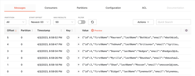
Now that we have our Kafka Connect worker up and running, let’s start streaming some data to our test topic. To do this, navigate to http://localhost:8080/topics. This will bring up the RedPanda UI with our test topic.

So click Actions -> Publish messages and publish the messages one by one from the JSONs below
As you send messages to the topic, you should see them appear in the topic’s message log. This confirms that your messages are being successfully produced and stored in the topic with partition 0.

Next, we can access MiniIO by going to http://localhost:9001/login using the login credentials “minioadmin” for both the username and password. In MiniIO, we will find the “my-bucket” bucket, which contains the sent messages that we streamed. The messages are stored in two files located under my-bucket/topics/test/partition=0/.

Remember when we set the Kafka Connect S3 Sync property “flush.size” to 3? That’s why there are two files in the my-bucket/topics/test/partition=0/ directory. Since we sent a total of 6 messages, each file contains 3 messages inside. You can download the files from MinIO to confirm that they contain the same data we sent to the RedPanda topic.
Let’s bring our containers down and look at another partitioning case.
docker-compose -f docker-compose.yml -f local/json-nonpartitioned-to-json/docker-compose.yml downField partitioner
Kafka Connect is a great tool for partitioning data output by specific fields. However, this feature requires structured data types, which means that input messages must have a schema. If you’re using Protobuf or Avro formats, you’ll need to set up a schema registry, which we’ll cover later. But if you don’t want to use a schema registry and deal with the schema management overhead, you can use JSON format with a schema. In this case, you would include the schema definition in the JSON message itself, and the Kafka Connect S3 sink connector can partition the output data without the need for a schema registry. This option is the easiest one to set up and use, but keep in mind that it might not be suitable for every use case, especially when you need to deal with complex data types or use different serialization formats.
As an example, I took one message from the DefaultPartitioner case and added a JSON schema, you can see it below. Also you can find all those JSONs with their schemas in my repo.
Let’s see how connector with field partitioner looks like.
You may have noticed that we made some changes to the environment variables, such as setting CONNECT_VALUE_CONVERTER_SCHEMAS_ENABLE to “true”. This means that our messages now have a schema attached to them. Additionally, we added new properties to the connector creation because we want to partition the output data by two fields: company and country. This is done using the FieldPartitioner. The “schema.generator.class” property specifies the schema generator to use, while the “partitioner.class” property specifies the partitioner to use. Finally, we set the “partition.field.name” property to “company,country” to indicate which fields to use for partitioning.
"schema.generator.class": "io.confluent.connect.storage.hive.schema.DefaultSchemaGenerator",
"partitioner.class": "io.confluent.connect.storage.partitioner.FieldPartitioner",
"value.converter.schemas.enable": "true",
"partition.field.name" : "company,country"
Let’s run containers with a new yaml file.
docker-compose -f docker-compose.yml -f local/json-partitioned-to-json/docker-compose.yml up -dTo follow the same algorithm, you should:
- Open the RedPanda console http://localhost:8080/topics
- Publish JSONs with schema

3. Open our bucket at http://localhost:9001/login with the username and password “minioadmin”.
You will see that the files are now organized and partitioned based on the company and country fields in the bucket.


So in the end of streaming you will get the next files:
my-bucket/warehouse/test/company=Block Group/country=Argentina/test+0+0000000000.json
my-bucket/warehouse/test/company=Block Group/country=France/test+0+0000000002.json
my-bucket/warehouse/test/company=Bruen-Donnelly/country=Indonesia/test+0+0000000004.json
my-bucket/warehouse/test/company=Hauck, Little and Hand/country=France/test+0+0000000005.json
my-bucket/warehouse/test/company=O'Keefe, O'Conner and Ullrich/country=France/test+0+0000000001.json
my-bucket/warehouse/test/company=Wintheiser, Sanford and Gusikowski/country=Peru/test+0+0000000003.json
If you set “partition.field.name” to “country,company”, then the file path will first have countries and then companies.
Let’s bring our containers down and look at the similar case when we want to do partitioning by time field.
docker-compose -f docker-compose.yml -f local/json-partitioned-to-json/docker-compose.yml downTime partitioner
What if we want to keep files according to some timestamp. We should use TimeBasedPartitioner. To see how it works, take a look at the connector container below.
You can see a set of new properties here.
"partitioner.class": "io.confluent.connect.storage.partitioner.TimeBasedPartitioner",
"path.format" : "'\'year\''=YYYY/'\'month\''=MM/'\'day\''=dd/'\'hour\''=HH",
"timestamp.extractor" : "RecordField",
"timestamp.field" : "login_timestamp",
"partition.duration.ms": "60000",
"locale": "en-US",
"timezone": "UTC"
The timestamp.extractor configuration property in Kafka determines how to get the timestamp from each record. By default, it uses the system time when the record is processed, but there are other options available. For example, it can use the timestamp of the Kafka record, which denotes when it was produced or stored by the broker. Additionally, you can extract the timestamp from one of the fields in the record's value by specifying the timestamp.field configuration property which is our case.
Let’s run the containers.
docker-compose -f docker-compose.yml -f local/json-partitioned-to-json/docker-compose-time.yml up -dWe can see that output files in our MinIO bucket are now partitioned based on the year, month, day, and hour. This partitioning is achieved by the path format that we have specified in our configuration, which is “‘’year’’=YYYY/’’month’’=MM/’’day’’=dd/’’hour’’=HH”.

And you get the next files:
my-bucket/warehouse/test/year=2022/month=01/day=19/hour=18/test+0+0000000003.json
my-bucket/warehouse/test/year=2022/month=03/day=22/hour=10/test+0+0000000000.json
my-bucket/warehouse/test/year=2022/month=04/day=25/hour=21/test+0+0000000004.json
my-bucket/warehouse/test/year=2022/month=05/day=05/hour=23/test+0+0000000002.json
my-bucket/warehouse/test/year=2022/month=07/day=14/hour=09/test+0+0000000005.json
my-bucket/warehouse/test/year=2022/month=10/day=23/hour=16/test+0+0000000001.json
What if you want to partition by field and time? Kafka Connect doesn’t support field and time separation together, but I found this repo which might work as a solution.
Don’t forget to stop our containers before we will look at more complicated case in the next chapter
docker-compose -f docker-compose.yml -f local/json-partitioned-to-json/docker-compose-time.yml downComplicated case — Confluent Schema Registry and Parquet
What if we decide to put on our grown-up pants and work with formats that require a little more sophistication?
Well, let’s be honest, JSON is great for small and simple data structures, but when it comes to serious data streaming, it’s not the most efficient and secure choice out there. It’s like bringing a bicycle to a Formula 1 race. That’s where Protobuf comes in handy, with its compact binary format that saves on network bandwidth and storage space. Plus, it provides a strong typing system, making it less prone to errors and more secure. So, if you want to step up your data streaming game, leave the bicycle at home and give Protobuf a try.
However, Protobuf requires a schema to be defined, and this is where we need Schema Registry. We will use a separate container running Schema Registry to manage the Protobuf schemas. We chose Confluent Schema Registry for this setup, but any other service with a Kafka API schema-registry endpoint can be used (for example, RedPanda schema registry). Additionally, we will use Parquet as the output format for the S3 bucket, which is one of the supported formats by Kafka Connect S3 Sink.
Here, in the image below, you can see our new team player in a pink rectangle.

This code block below shows the changes we made to our connector configuration. We added a new property for the Protobuf converter with the schema registry URL so that the converter can look up the schema for the data it’s processing. We also set “schemas.enable” to false to disable the Avro schema that’s used by default.
CONNECT_VALUE_CONVERTER: io.confluent.connect.protobuf.ProtobufConverter
CONNECT_VALUE_CONVERTER_SCHEMA_REGISTRY_URL: "http://schema-registry:8081"
CONNECT_VALUE_CONVERTER_SCHEMAS_ENABLE: "false"
Additionally, the partitioner class is “FieldPartitioner” as in our second case and we set Parquet format as the output format for our S3 bucket and set the codec to “gzip” for compression.
Finally, we set the value subject name strategy to “RecordNameStrategy” to use the name of the Protobuf message as the subject name in the schema registry. All these changes will ensure that our connector is using Protobuf format and partitioning the data properly while storing it in the S3 bucket.
"value.converter.schemas.enable": "false",
"value.converter": "io.confluent.connect.protobuf.ProtobufConverter",
"value.converter.schema.registry.url": "http://schema-registry:8081",
"partitioner.class": "io.confluent.connect.storage.partitioner.FieldPartitioner",
"value.converter.value.subject.name.strategy": "io.confluent.kafka.serializers.subject.RecordNameStrategy",
"partition.field.name" : "company,country",
"format.class": "io.confluent.connect.s3.format.parquet.ParquetFormat",
"parquet.codec": "gzip"
Let’s run our containers. You might notice a new container here — schema registry.
docker-compose -f docker-compose.yml  -f local/json-schema-registry/docker-compose.yml up -d

docker ps
So it’s time to create our Protobuf schema. Protobuf schema is a way to define the structure of your data in a language-agnostic way, using Google’s Protocol Buffers. It’s like a blueprint for your data that allows you to define the fields, types, and structure of your data. This way, your data can be easily serialized and deserialized between different programming languages and platforms. I used some online tool to create the schema from the tutorial JSONs.
syntax = "proto3";

message User{
uint32 id = 1;
string first_name = 2;
string last_name = 3;
string email = 4;
string login_timestamp = 5;
string ip_address = 6;
string country = 7;
string company = 8;
}
Then we should wrap it into JSON file, which we call protobuf-schema.json, and use curl to create a new version of User schema in our Schema Registry.
curl -X POST -H "Content-Type: application/vnd.schemaregistry.v1+json" \
  --data-binary @local/json-schema-registry/protobuf-schema.json \
  http://localhost:8081/subjects/User/versions
This curl command above is creating a new version of a Protobuf schema named User in a Schema Registry service endpoint running at http://localhost:8081.
The command is sending a POST request with the Protobuf schema data, which is specified by the --data-binary flag with the path to the our file local/json-schema-registry/protobuf-schema.json. The Content-Type header is set to application/vnd.schemaregistry.v1+json, indicating that the data is in JSON format and the API version of the schema registry being used.
The Schema Registry service will validate the schema and store it. The response from the service will contain the ID of the schema version that was created. This ID will be used to reference the schema when configuring Kafka Connect.
You can see the schema in RedPanda console. You might notice that schema ID is 1 here, we will use this value later for Protobuf producer.

When working with Protobuf data, there are various options for producers. You can either use an existing Protobuf producer or write your own. However, to keep things simple, we will be using the kafka-protobuf-console-producer in this case. It is designed to produce Protobuf messages from the console input and send them to a Kafka topic. You can use it from the command line, making it easy to get started with producing Protobuf data because it can serialize our JSON messages using our schema from schema-registry.
Let’s start. This command below will run a protobuf console producer in a Docker container. The producer will send messages to our RedPanda topic named test. The producer will also use a Protobuf schema from the Schema Registry service running on the “schema-registry” container, specified by the property “schema.registry.url”. The property “value.schema.id” specifies the ID of the Protobuf schema to be used, which is 1 in this case.
docker exec -it schema-registry kafka-protobuf-console-producer --bootstrap-server redpanda:9092 --property value.schema.id="1" --property schema.registry.url="http://schema-registry:8081" --topic testThen you should send our JSON messages in the command line one by one

In Kafka, messages are usually serialized before being sent to topics, and deserialized before being consumed by consumers. Protobuf messages are also serialized and deserialized in the same way. However, since we have enabled the schema-registry with Protobuf support in the Console container, it means that the Console is now aware of our User protobuf schema.
schemaRegistry:
    enabled: true
    urls: ["http://redpanda:8081"]
protobuf:
  enabled: true
  schemaRegistry:
    enabled: true
    refreshInterval: 5m
This allows the console to automatically deserialize the messages received from the topic using our protobuf schema, making them more human-readable. This means that we can now see the messages on the topic in a deserialized way without having to manually deserialize them ourselves. This makes it easier to understand and analyze the data flowing through the RedPanda topic.
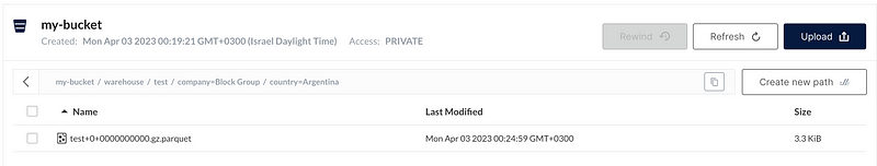
We have configured the Sink to partition the data based on the company and country fields, similar to our second use case. However, this time we have chosen Parquet as the output format for the S3 bucket. As a result, when we look at the files in MinIO, we can see that they are partitioned based on the specified fields and the format of the files is Parquet.
Conclusion
Well folks, we’ve come to the end of this tutorial on streaming data from Kafka to Amazon S3. We’ve covered everything from setting up your local environment with Docker Desktop on MacOS to real streaming using RedPanda, Kafka Connect and MinIO. And let’s not forget about the exciting world of partitioning your data for even better performance and analysis! Who knew data streaming could be so thrilling? But in all seriousness, with the power of Kafka and the flexibility of S3, you can create some truly amazing data applications that will make all your colleagues jealous.